Theoretical material on the modules "probability theory and mathematical statistics". Great encyclopedia of oil and gas

Problem 14. In the cash lottery, 1 win of 1,000,000 rubles, 10 wins of 100,000 rubles are played. and 100 wins of 1000 rubles each. with a total number of tickets of 10,000. Find the law of distribution of random winnings X for the owner of one lottery ticket.

Solution. Possible values for X: X 1 = 0; X 2 = 1000; X 3 = 100000;

X 4 = 1000000. Their probabilities are respectively equal: R 2 = 0,01; R 3 = 0,001; R 4 = 0,0001; R 1 = 1 – 0,01 – 0,001 – 0,0001 = 0,9889.

Therefore, the law of distribution of winnings X can be given by the following table:

Problem 15. Discrete random variable X is given by the distribution law:

Construct a distribution polygon.

Solution. Let's build a rectangular coordinate system, and we'll plot possible values along the abscissa axis x i, and along the y-axis - the corresponding probabilities p i. Let's plot the points M 1 (1;0,2), M 2 (3;0,1), M 3 (6;0.4) and M 4 (8;0.3). By connecting these points with straight line segments, we obtain the desired distribution polygon.

§2. Numerical characteristics of random variables

A random variable is completely characterized by its distribution law. An averaged description of a random variable can be obtained by using its numerical characteristics

2.1. Expected value. Dispersion.

Let a random variable take values with probabilities accordingly.

Definition. The mathematical expectation of a discrete random variable is the sum of the products of all its possible values and the corresponding probabilities:

Properties of mathematical expectation.

The dispersion of a random variable around the mean value is characterized by dispersion and standard deviation.

The variance of a random variable is the mathematical expectation of the squared deviation of a random variable from its mathematical expectation:

The following formula is used for calculations

Properties of dispersion.

2. , where are mutually independent random variables.

3. Standard deviation.

Problem 16. Find the mathematical expectation of a random variable Z = X+ 2Y, if the mathematical expectations of random variables are known X And Y: M(X) = 5, M(Y) = 3.

Solution. We use the properties of mathematical expectation. Then we get:

M(X+ 2Y)= M(X) + M(2Y) = M(X) + 2M(Y) = 5 + 2 . 3 = 11.

Problem 17. Variance of a random variable X is equal to 3. Find the variance of random variables: a) –3 X; b) 4 X + 3.

Solution. Let's apply properties 3, 4 and 2 of dispersion. We have:

A) D(–3X) = (–3) 2 D(X) = 9D(X) = 9 . 3 = 27;

b) D(4X+ 3) = D(4X) + D(3) = 16D(X) + 0 = 16 . 3 = 48.

Problem 18. Given an independent random variable Y– the number of points obtained when throwing a die. Find the distribution law, mathematical expectation, dispersion and standard deviation of a random variable Y.

Solution. Random variable distribution table Y has the form:

Then M(Y) = 1 1/6 + 2 1/6 + 3 1/6+ 4 1/6+ 5 1/6+ 6 1/6 = 3.5;

D(Y) = (1 – 3.5) 2 1/6 +(2 – 3.5) 2 /6 + (3 – 3.5) 2 1/6 + (4 – 3.5) 2 / 6 +(5 – –3.5) 2 1/6 + (6 – 3.5) 2. 1/6 = 2.917; σ (Y) =Ö 2,917 = 1,708.

Random variables: discrete and continuous.

When conducting a stochastic experiment, a space of elementary events is formed - possible outcomes of this experiment. It is believed that on this space of elementary events there is given random value X, if a law (rule) is given according to which each elementary event is associated with a number. Thus, the random variable X can be considered as a function defined on the space of elementary events.

■ Random variable- a quantity that, during each test, takes on one or another numerical value (it is not known in advance which one), depending on random reasons that cannot be taken into account in advance. Random variables are denoted by capital letters of the Latin alphabet, and possible values of a random variable are denoted by small letters. So, when throwing a die, an event occurs associated with the number x, where x is the number of points rolled. The number of points is a random variable, and the numbers 1, 2, 3, 4, 5, 6 are possible values of this value. The distance that a projectile will travel when fired from a gun is also a random variable (depending on the installation of the sight, the strength and direction of the wind, temperature and other factors), and the possible values of this value belong to a certain interval (a; b).

■ Discrete random variable– a random variable that takes on separate, isolated possible values with certain probabilities. The number of possible values of a discrete random variable can be finite or infinite.

■ Continuous random variable– a random variable that can take all values from some finite or infinite interval. The number of possible values of a continuous random variable is infinite.

For example, the number of points rolled when throwing a dice, the score for a test are discrete random variables; the distance that a projectile flies when firing from a gun, the measurement error of the indicator of time to master educational material, the height and weight of a person are continuous random variables.

Distribution law of a random variable– correspondence between possible values of a random variable and their probabilities, i.e. Each possible value x i is associated with the probability p i with which the random variable can take this value. The distribution law of a random variable can be specified tabularly (in the form of a table), analytically (in the form of a formula), and graphically.

Let a discrete random variable X take values x 1 , x 2 , …, x n with probabilities p 1 , p 2 , …, p n respectively, i.e. P(X=x 1) = p 1, P(X=x 2) = p 2, …, P(X=x n) = p n. When specifying the distribution law of this quantity in a table, the first row of the table contains possible values x 1 , x 2 , ..., x n , and the second row contains their probabilities

X	x 1	x 2	…	x n
p	p 1	p2	…	p n

As a result of the test, a discrete random variable X takes on one and only one of the possible values, therefore the events X=x 1, X=x 2, ..., X=x n form a complete group of pairwise incompatible events, and, therefore, the sum of the probabilities of these events is equal to one , i.e. p 1 + p 2 +… + p n =1.

Distribution law of a discrete random variable. Distribution polygon (polygon).

As you know, a random variable is a variable that can take on certain values depending on the case. Random variables are denoted by capital letters of the Latin alphabet (X, Y, Z), and their values are denoted by corresponding lowercase letters (x, y, z). Random variables are divided into discontinuous (discrete) and continuous.

A discrete random variable is a random variable that takes only a finite or infinite (countable) set of values with certain non-zero probabilities.

Distribution law of a discrete random variable is a function that connects the values of a random variable with their corresponding probabilities. The distribution law can be specified in one of the following ways.

1. The distribution law can be given by the table:

where λ>0, k = 0, 1, 2, … .

c) using the distribution function F(x), which determines for each value x the probability that the random variable X will take a value less than x, i.e. F(x) = P(X< x).

Properties of the function F(x)

3. The distribution law can be specified graphically - by a distribution polygon (polygon) (see task 3).

Note that to solve some problems it is not necessary to know the distribution law. In some cases, it is enough to know one or several numbers that reflect the most important features of the distribution law. This can be a number that has the meaning of the “average value” of a random variable, or a number showing the average size of the deviation of a random variable from its mean value. Numbers of this kind are called numerical characteristics of a random variable.

Basic numerical characteristics of a discrete random variable:

Mathematical expectation (average value) of a discrete random variable M(X)=Σ x i p i .
For binomial distribution M(X)=np, for Poisson distribution M(X)=λ
Dispersion of a discrete random variable D(X)= M 2 or D(X) = M(X 2)− 2. The difference X–M(X) is called the deviation of a random variable from its mathematical expectation.
For binomial distribution D(X)=npq, for Poisson distribution D(X)=λ
Mean square deviation (standard deviation) σ(X)=√D(X).

· For clarity of presentation of a variation series, its graphic images are of great importance. Graphically, a variation series can be depicted as a polygon, histogram and cumulate.

· A distribution polygon (literally a distribution polygon) is called a broken line, which is constructed in a rectangular coordinate system. The value of the attribute is plotted on the abscissa, the corresponding frequencies (or relative frequencies) - on the ordinate. Points (or) are connected by straight line segments and a distribution polygon is obtained. Most often, polygons are used to depict discrete variation series, but they can also be used for interval series. In this case, the points corresponding to the midpoints of these intervals are plotted on the abscissa axis.

Solution. Possible values for X: X 1 = 0; X 2 = 1000; X 3 = 100000;

X 4 = 1000000. Their probabilities are respectively equal: R 2 = 0,01; R 3 = 0,001; R 4 = 0,0001; R 1 = 1 – 0,01 – 0,001 – 0,0001 = 0,9889.

Therefore, the law of distribution of winnings X can be given by the following table:

Construct a distribution polygon.

§2. Numerical characteristics of random variables

A random variable is completely characterized by its distribution law. An averaged description of a random variable can be obtained by using its numerical characteristics

2.1. Expected value. Dispersion.

Let a random variable take values with probabilities accordingly.

Definition. The mathematical expectation of a discrete random variable is the sum of the products of all its possible values and the corresponding probabilities:

Properties of mathematical expectation.

The dispersion of a random variable around the mean value is characterized by dispersion and standard deviation.

The variance of a random variable is the mathematical expectation of the squared deviation of a random variable from its mathematical expectation:

The following formula is used for calculations

Properties of dispersion.

2. , where are mutually independent random variables.

3. Standard deviation .

Problem 16. Find the mathematical expectation of a random variable Z = X+ 2Y, if the mathematical expectations of random variables are known X And Y: M(X) = 5, M(Y) = 3.

Solution. We use the properties of mathematical expectation. Then we get:

M(X+ 2Y)= M(X) + M(2Y) = M(X) + 2M(Y) = 5 + 2 . 3 = 11.

Problem 17. Variance of a random variable X is equal to 3. Find the variance of random variables: a) –3 X; b) 4 X + 3.

Solution. Let's apply properties 3, 4 and 2 of dispersion. We have:

A) D(–3X) = (–3) 2 D(X) = 9D(X) = 9 . 3 = 27;

b) D(4X+ 3) = D(4X) + D(3) = 16D(X) + 0 = 16 . 3 = 48.

Solution. Random variable distribution table Y has the form:

Y
R	1/6	1/6	1/6	1/6	1/6	1/6

Then M(Y) = 1 1/6 + 2 1/6 + 3 1/6+ 4 1/6+ 5 1/6+ 6 1/6 = 3.5;

D(Y) = (1 – 3.5) 2 1/6 +(2 – 3.5) 2 /6 + (3 – 3.5) 2 1/6 + (4 – 3.5) 2 / 6 +(5 – –3.5) 2 1/6 + (6 – 3.5) 2. 1/6 = 2.917; σ (Y) =Ö 2,917 = 1,708.

Discrete called a random variable that can take on separate, isolated values with certain probabilities.

EXAMPLE 1. The number of times the coat of arms appears in three coin tosses. Possible values: 0, 1, 2, 3, their probabilities are equal respectively:

P(0) = ; Р(1) = ; Р(2) = ; Р(3) = .

EXAMPLE 2. The number of failed elements in a device consisting of five elements. Possible values: 0, 1, 2, 3, 4, 5; their probabilities depend on the reliability of each element.

Discrete random variable X can be given by a distribution series or a distribution function (the integral distribution law).

Near distribution is the set of all possible values Xi and their corresponding probabilities Ri = P(X = xi), it can be specified as a table:

x i				x n
p i				р n

At the same time, the probabilities Ri satisfy the condition

Ri= 1 because

where is the number of possible values n may be finite or infinite.

Graphical representation of the distribution series called the distribution polygon . To construct it, possible values of the random variable ( Xi) are plotted along the x-axis, and the probabilities Ri- along the ordinate axis; points Ai with coordinates ( Xi,рi) are connected by broken lines.

Distribution function random variable X called function F(X), whose value at the point X is equal to the probability that the random variable X will be less than this value X, that is

F(x) = P(X< х).

Function F(X) For discrete random variable calculated by the formula

F(X) = Ri , (1.10.1)

where the summation is carried out over all values i, for which Xi< х.

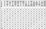
EXAMPLE 3. From a batch containing 100 products, of which there are 10 defective, five products are randomly selected to check their quality. Construct a series of distributions of a random number X defective products contained in the sample.

Solution. Since in the sample the number of defective products can be any integer ranging from 0 to 5 inclusive, then the possible values Xi random variable X are equal:

x 1 = 0, x 2 = 1, x 3 = 2, x 4 = 3, x 5 = 4, x 6 = 5.

Probability R(X = k) that the sample contains exactly k(k = 0, 1, 2, 3, 4, 5) defective products, equals

P (X = k) = .

As a result of calculations using this formula with an accuracy of 0.001, we obtain:

R 1 = P(X = 0) @ 0,583;R 2 = P(X = 1) @ 0,340;R 3 = P(X = 2) @ 0,070;

R 4 = P(X = 3) @ 0,007;R 5 = P(X= 4) @ 0;R 6 = P(X = 5) @ 0.

Using equality to check Rk=1, we make sure that the calculations and rounding were done correctly (see table).

x i
p i

EXAMPLE 4. Given a distribution series of a random variable X :

x i
p i

Find the probability distribution function F(X) of this random variable and construct it.

Solution. If X£10 then F(X)= P(X<X) = 0;

if 10<X£20 then F(X)= P(X<X) = 0,2 ;

if 20<X£30 then F(X)= P(X<X) = 0,2 + 0,3 = 0,5 ;

if 30<X£40 then F(X)= P(X<X) = 0,2 + 0,3 + 0,35 = 0,85 ;

if 40<X£50 then F(X)= P(X<X) = 0,2 + 0,3 + 0,35 + 0,1=0,95 ;

If X> 50, then F(X)= P(X<X) = 0,2 + 0,3 + 0,35 + 0,1 + 0,05 = 1.

Random variable is a quantity that, as a result of experiment, can take on one or another value that is not known in advance. There are random variables discontinuous (discrete) And continuous type. Possible values of discontinuous quantities can be listed in advance. Possible values of continuous quantities cannot be listed in advance and continuously fill a certain gap.

Example of discrete random variables:

1) The number of times the coat of arms appears in three coin tosses. (possible values 0;1;2;3)

2) Frequency of appearance of the coat of arms in the same experiment. (possible values)

3) The number of failed elements in a device consisting of five elements. (Possible values 0;1;2;3;4;5)

Examples of continuous random variables:

1) Abscissa (ordinate) of the point of impact when fired.

2) Distance from the point of impact to the center of the target.

3) Uptime of the device (radio tube).

Random variables are denoted by capital letters, and their possible values are denoted by corresponding small letters. For example, X is the number of hits with three shots; possible values: X 1 =0, X 2 =1, X 3 =2, X 4 =3.

Let's consider a discontinuous random variable X with possible values X 1, X 2, ..., X n. Each of these values is possible, but not certain, and the value X can take each of them with some probability. As a result of the experiment, the value of X will take one of these values, that is, one of the complete group of incompatible events will occur.

Let us denote the probabilities of these events by the letters p with the corresponding indices:

Since incompatible events form a complete group, then

that is, the sum of the probability of all possible values of a random variable is equal to 1. This total probability is somehow distributed among the individual values. A random variable will be fully described from a probabilistic point of view if we define this distribution, that is, we indicate exactly what probability each of the events has. (This will establish the so-called law of distribution of random variables.)

Law of distribution of a random variable is any relation that establishes a connection between the possible values of a random variable and the corresponding probability. (We will say about a random variable that it is subject to a given distribution law)

The simplest form of specifying the distribution law of a random variable is a table that lists the possible values of the random variable and the corresponding probabilities.

Table 1.

X i	X 1	X 2	…	Xn
P i	P 1	P2	…	Pn

This table is called near distribution random variables.

To give the distribution series a more visual appearance, they resort to its graphical representation: the possible values of the random variable are plotted along the abscissa axis, and the probabilities of these values are plotted along the ordinate axis. (For clarity, the resulting points are connected by straight line segments.)

Figure 1 – distribution polygon

This figure is called distribution polygon. The distribution polygon, like the distribution series, completely characterizes the random variable; it is one of the forms of the law of distribution.

Example:

one experiment is performed in which event A may or may not appear. The probability of event A = 0.3. We consider a random variable X - the number of occurrences of event A in a given experiment. It is necessary to construct a series and polygon of the distribution of the X value.

Table 2.

X i
P i	0,7	0,3

Figure 2 - Distribution function

Distribution function is a universal characteristic of a random variable. It exists for all random variables: both discontinuous and non-continuous. The distribution function fully characterizes a random variable from a probabilistic point of view, that is, it is one of the forms of the distribution law.

To quantitatively characterize this probability distribution, it is convenient to use not the probability of event X=x, but the probability of event X

The distribution function F(x) is sometimes also called the cumulative distribution function or the cumulative distribution law.

Properties of the distribution function of a random variable

1. The distribution function F(x) is a non-decreasing function of its argument, that is, for ;

2. At minus infinity:

3. On plus infinity:

Figure 3 – distribution function graph

Distribution function graph in general, it is a graph of a non-decreasing function whose values start from 0 and go to 1.

Knowing the distribution series of a random variable, it is possible to construct the distribution function of the random variable.

Example:

for the conditions of the previous example, construct the distribution function of the random variable.

Let's construct the distribution function X:

Figure 4 – distribution function X

Distribution function of any discontinuous discrete random variable there is always a discontinuous step function, the jumps of which occur at points corresponding to the possible values of the random variable and are equal to the probabilities of these values. The sum of all distribution function jumps is equal to 1.

As the number of possible values of a random variable increases and the intervals between them decrease, the number of jumps becomes larger, and the jumps themselves become smaller:

Figure 5

The stepped curve becomes smoother:

Figure 6

The random variable gradually approaches a continuous value, and its distribution function approaches a continuous function. There are also random variables whose possible values continuously fill a certain interval, but for which the distribution function is not continuous everywhere. And at certain points it breaks. Such random variables are called mixed.

Figure 7